Binary Junction by Pure Python
We can run the following test case without having to compile OpenDiS.
To run the simulation, simply execute:
cd ${OPENDIS_DIR}
cd examples/03_binary_junction
python3 -i test_binary_junction_pydis.py
Initial Condition
The initial configuration for this simulation is made of two dislocation lines intersecting at a single point. Each dislocation line consists of three nodes, and their end nodes are pinned (constraint == PINNED_NODE). On the other hand, nodes in the middle of the lines are unconstrained. This allows the two dislocation lines to form a binary junction under zero stress condition.
Boundary Condition
Periodic boundary condition (PBC) is turned off, as specified in the following line of the test script.
net = init_two_disl_lines(z0=z0, box_length=Lbox, pbc=False)
Simulation Behavior
If the simulation runs successfully, a (Python Matplotlib) window should open and the final dislocation configuration at the end of the simulation should look something like this.
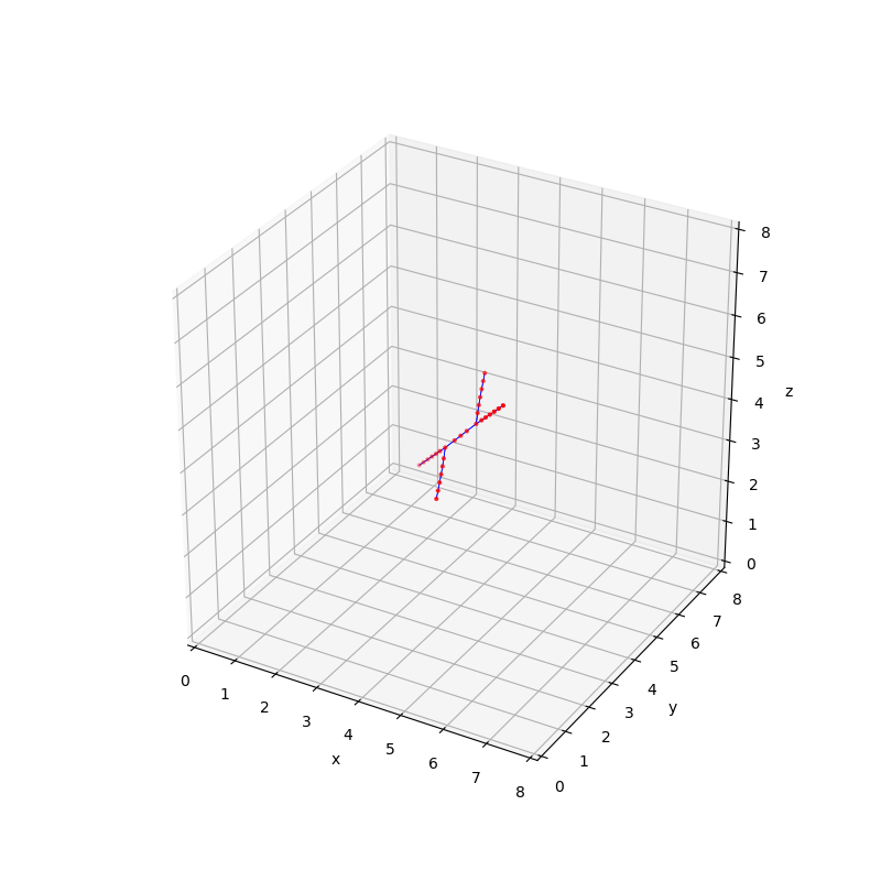
Here is what you should see during the simulation.
Hint
If you do not see a new window displaying the dislocation configuration, it is possible because you are running on a remote server and didn’t have the X11 forwarding set up correctly.
Add the -Y option in your ssh command, such as ssh -Y <your_account>@your.cluster.address. You can also try the xeyes command (which will open a new window) to verify that your X11 channel is set up correctly.
Dislocation Network Examination
Since we ran the test case in Python interactive mode (with the -i option), we can examine the data structure representing the dislocation network (i.e. a graph) at the end of the simulation. For example, use the following command to see all the nodes (DisNode) in the dislocation network (DisNet).
G.all_nodes_tags()
Each node is labeled by a tag, which is a tuple of two integers, (domainID, index). This is following the convention of ParaDiS. In this example, the domainID equals 0 for all nodes. The output of the above command is
dict_keys([(0, 0), (0, 2), (0, 3), (0, 4), (0, 5), (0, 1), (0, 6), (0, 7), (0, 8), (0, 9), (0, 10), (0, 12), (0, 14), (0, 15), (0, 18), (0, 19), (0, 21), (0, 22), (0, 23), (0, 25), (0, 26), (0, 27), (0, 28), (0, 29), (0, 31), (0, 33), (0, 24), (0, 30), (0, 20)])
To examine the information (i.e. attributes) of a node, use the following command, e.g.
G.nodes((0,0)).view()
The output is
{'R': array([4., 3., 3.]), 'constraint': 7}
Use the following command to see all the segments (DisEdge) in the dislocation network (DisNet).
list(G.all_segments_tags())
The output of the above command is
[((0, 3), (0, 18)), ((0, 18), (0, 10)), ((0, 10), (0, 19)), ((0, 19), (0, 1)), ((0, 21), (0, 6)), ((0, 6), (0, 22)), ((0, 22), (0, 12)), ((0, 12), (0, 23)), ((0, 23), (0, 5)), ((0, 25), (0, 7)), ((0, 7), (0, 26)), ((0, 26), (0, 14)), ((0, 14), (0, 27)), ((0, 27), (0, 2)), ((0, 8), (0, 28)), ((0, 28), (0, 15)), ((0, 15), (0, 29)), ((0, 29), (0, 0)), ((0, 31), (0, 8)), ((0, 33), (0, 1)), ((0, 4), (0, 30)), ((0, 30), (0, 24)), ((0, 24), (0, 20)), ((0, 20), (0, 9)), ((0, 9), (0, 33)), ((0, 25), (0, 4)), ((0, 31), (0, 9)), ((0, 21), (0, 4))]
We can see that each segment is specified by the tags of its two end nodes. Each segment is included only once in this representation.
To examine the information (i.e. attributes) of a segment, use the following command, e.g.
G.segments(((0, 3), (0, 18))).view()
The output is
{'source_tag': (0, 3), 'target_tag': (0, 18), 'burg_vec': array([ 1., -1., 1.]), 'plane_normal': array([-0.70710678, 0. , 0.70710678])}
Note that each segment needs to know the line direction corresponding to the Burgers vector being stored. The line direction goes from the node designated by source_tag.
We can use the burg_vec_from function to obtain the Burgers vector using either one of the two end nodes, e.g.
G.segments(((0, 3), (0, 18))).burg_vec_from((0, 3))
The output is
array([ 1., -1., 1.])
Alternatively,
G.segments(((0, 3), (0, 18))).burg_vec_from((0, 18))
The output is
array([-1., 1., -1.])
We can also examine the information for the simulation cell as follows
G.cell.view()
The output of the above command is,
{'h': array([[8., 0., 0.],
       [0., 8., 0.],
       [0., 0., 8.]]), 'hinv': array([[0.125, 0.   , 0.   ],
       [0.   , 0.125, 0.   ],
       [0.   , 0.   , 0.125]]), 'origin': array([0., 0., 0.]), 'is_periodic': [False, False, False]}